Iterative Methods

Iterative Methods

Why do we need another method to solve a set of simultaneous linear equations?

In certain cases, such as when a system of equations is large, iterative methods of solving equations are more advantageous. Elimination methods, such as Gaussian elimination, are prone to large round-off errors for a large set of equations. Iterative methods, give the user control of the round-off error. Also, if the physics of the problem are well known, initial guesses needed in iterative methods can be made more judiciously leading to faster convergence.

Jacobi's Method

The Jacobi method is a method of solving a matrix equation on a matrix that has no zeros along its main diagonal. Each diagonal element is solved for, and an approximate value plugged in. The process is then iterated until it converges.

The Jacobi method is easily derived by examining each of the n equations in the linear system of equations Ax = b in isolation. If, in the i-th equation:

Solve for the value of Xi while assuming the other entries of x remain fixed. This suggests an iterative method:

In this method, the order in which the equations are examined is irrelevant, since the Jacobi method treats them independently. The definition of the Jacobi method can be expressed with matrices as:

References:

http://mathworld.wolfram.com/JacobiMethod.html

http://www.nhcue.edu.tw/~jinnliu/teaching/nde07/Lecture3.pdf

Gauss-Seidel Method

The Gauss-Seidel method is a technique used to solve a linear system of equations.

The method is similar to the Jacobi method and in the same way strict or irreducible diagonal dominance of the system is sufficient to ensure convergence, meaning the method will work.

Procedure:

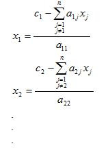
If the diagonal elements are non-zero, each equation is rewritten for the corresponding unknown, that is, the first equation is rewritten with X1 on the left hand side, the second equation is rewritten with X2 on the left hand side and so on.

The equations can be rewritten in summaration form as:

Now to find Xi’s, one assumes an initial guess for the Xi’s and then uses the rewritten equations to calculate the new estimates. Remember, one always uses the most recent estimates to calculate the next estimates, Xi. At the end of each iteration, one calculates the absolute relative approximate error for each Xi.

Important: Remember to use the most recent value of xi. Which means to apply values calculated to the calculations remaining in the current iteration.

Example:

Refrences:

http://numericalmethods.eng.usf.edu/topics/gauss_seidel.html

http://www.cfd-online.com/Wiki/Gauss-Seidel_method

Successive Overrelaxation Method (SOR)

The successive overrelaxation method (SOR) is a method of solving a linear system of equations derived by extrapolating the Gauss-Seidel method. This extrapolation takes the form of a weighted average between the previous iterate and the computed Gauss-Seidel iterate successively for each component,

where denotes a Gauss-Seidel iterate and is the extrapolation factor. The idea is to choose a value for that will accelerate the rate of convergence of the iterates to the solution.

In matrix terms, the SOR algorithm can be written as

where the matrices D, -L, and -U represent the diagonal, strictly lower-triangular, and strictly upper-triangular parts of A, respectively.

, the SOR method simplifies to the Gauss-Seidel method. A theorem due to Kahan (1958) shows that SOR fails to converge if

is outside the interval (0,2).

In general, it is not possible to compute in advance the value of

that will maximize the rate of convergence of SOR. Frequently, some heuristic estimate is used, such as

where

is the mesh spacing of the discretization of the underlying physical domain.

References:

http://mathworld.wolfram.com/SuccessiveOverrelaxationMethod.html

http://math.fullerton.edu/mathews/n2003/SORmethodMod.html

Linear Algebraic Equations

Gaussian Elimination

One of the most popular techniques for solving simultaneous linear equations is the Gaussian elimination method. The approach is designed to solve a general set of n equations and n unknowns.

Gaussian elimination consists in these two steps:

Forward Elimination of Unknowns:

In the first step of forward elimination, the first unknown, x1 is eliminated from all rows below the first row. The first equation is selected as the pivot equation to eliminate x1. So, to eliminate x1 in the second equation, one multiplies the first equation by a21/a11 to give:

This procedure of eliminating x1, is now repeated for the third equation to the n-th equation to reduce the set of equations as:

This is the end of the first step of forward elimination. Now for the second step of forward elimination, we start with the second equation as the pivot equation and a'22 as the pivot element. So, to eliminate x2 in the third equation, by multiplying the second equation by a'32/a'22 and subtracting it from the third equation. This makes the coefficient of x2 zero in the third equation. The same procedure is now repeated for the fourth equation till the n-th equation to give:

The next steps of forward elimination are conducted by using the third equation as a pivot equation and so on. That is, there will be a total of n-1 steps of forward elimination.

Back Substitution:

Now the equations are solved starting from the last equation as it has only one unknown.

Then the second last equation, that is the (n-1)th equation, has two unknowns: Xn and Xn-1, but Xn is already known. This reduces the (n-1)th equation also to one unknown. Back substitution hence can be represented for all equations by the formula:

*Example Naive Gaussian Elimination: In the next two videos we can see the 2 steps of the method (explained before)

References:

Holistic Numerical Methods Institute - Gaussian Elimination

Gauss-Jordan Elimination

Gauss-Jordan Elimination is a variant of Gaussian Elimination. Again, we are transforming the coefficient matrix into another matrix that is much easier to solve, and the system represented by the new augmented matrix has the same solution set as the original system of linear equations. In Gauss-Jordan Elimination, the goal is to transform the coefficient matrix into a diagonal matrix, and the zeros are introduced into the matrix one column at a time. We work to eliminate the elements both above and below the diagonal element of a given column in one pass through the matrix.

Procedure:

Note: If you're unable to do step 2, stop! the system has either infinite or no solutions

Example:

It is now obvious, by inspection, that the solution to this linear system is x=3, y=1, and z=2. Again, by solution, it is meant the x, y, and z required to satisfy all the equations simultaneously.

References:

http://www.krellinst.org/AiS/textbook/unit2/example_projects/starter/math/matrix/gauss.html

http://ceee.rice.edu/Books/CS/chapter2/linear44.html

LU Descomposition

Another way of solving a system of equations is by using a factorization technique for matrices called LU decompostion. This factorization involves two matrices, one lower triangular matrix and one upper triangular matrix.

How to find an LU decomposition? Hints:

* To get the matrix U, just use row operations until an upper triangular matrix is formed.

* To get L, start with the idenity matrix and use the following rules. Any row operations that involves adding a multiple of one row to another, for example, Ri + kRj, put the value –k in the ith-row, jth-column of the identity matrix. Any row operations that involves getting a leading one on the main diagonal, for example, kRi, put the value 1/k in the position of the identity matrix where the leading one occurs.

Example: (Steps)

Find an LU decomposition of the following matrix.

1. Use Gaussian Elimination to get the upper triangular matrix U.

2. Form the lower triangular matrix L by using the rules mentioned above for the

row operations involved to get U.

Thus an LU Decomposition is given by

Next is shown how an LU decomposition can be used to solve a system of equations.

Steps to solve a system using an LU decomposition:

1. Set up the equation Ax = b.

2. Find an LU decomposition for A. This will yield the equation (LU)x = b.

3. Let y = Ux. Then solve the equation Ly = b for y.

4. Take the values for y and solve the equation y = Ux for x. This will give the solution to the system Ax = b.

Finally, in the next video we'll see another example, for more understanding of the LU method:

References:

http://www.utdallas.edu/dept/abp/PDF_Files/LinearAlgebra_Folder/LU_Decomposition.pdf

Videos:

* Theory For Gaussian Elimination With Partial Pivoting:

*Why? LU Descomposition

Root Of A Polynomial

Muller's Method

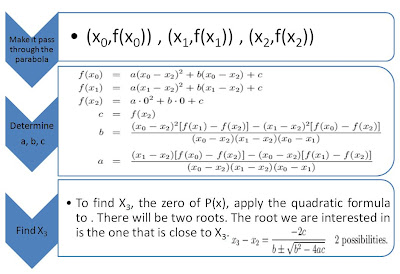
Muller's Method is a generalization of the secant method, in the sense that it does not require the derivate of the function. It is an iterative method that requires 3 starting points (xo, f(xo)) , (x1, f(x1)) , (x2, f(x2)). A parabola is constructed that passes through the three points; the quadratic formula is used to find a root of the quadratic for the next approximation. It has been proved that near a simple root Muller´s Method converges faster than the secant method and almost as fast as Newton's method. The method can be used to find real or complex zeros of a function and can be programed to use complex arithmetic.

The fact that this method can be used to find complex roots is one of the main advantages of Müller's method.

Comparison With Secant Method:

Procedure:
Consider $P(x)=a(x-x_2)^2+b(x-x_2)+c$
Once

x₃

is determined, let

x_o = x₁ , x₁ = x₂ , x₂ = x₃

and repeat.
Example:
Suppose we wish to find a root of the polynomial X7 + 3X6 + 7X5 + X4 + 5X3 + 2X2 + 5X + 5.
We will use Xo=0, X1=-0.1 and x2=-0.2 as our three numerical approximations. Tolerance = 0.0001
Results are shown in the next table:

Thus the last step, the tolerance is met, and therefore, after six iterations, our approximationto the root is -0.706826.

References:

http://math.arizona.edu/~restrepo/475A/Notes/sourcea/node25.html

http://math.fullerton.edu/mathews/n2003/MullersMethodMod.html

http://www.ece.uwaterloo.ca/~dwharder/NumericalAnalysis/10RootFinding/mueller/

Bairstow's Method

Bairstow Method is an iterative method used to find both the real and complex roots of a polynomial. It is based on the idea of synthetic division of the given polynomial by a quadratic function and can be used to find all the roots of a polynomial. Given a polynomial say

Bairstow's method divides the polynomial by a quadratic function: $\displaystyle x^{2}-rx-s.$

Now the quotient will be a polynomial: $\displaystyle f_{n-2}(x)=b_{2}+b_{3}x+b_{4}x^{2}+...+b_{n-1}x^{n-3}+b_{n}x^{n-2}$

and the remainder is a linear function: $\displaystyle R(x)=b_{1}(x-r)+b_{0}$

Since the quotient $f_{n-2}(x)$ and the remainder are obtained by standard synthetic division the co-efficients can be obtained by the following recurrence relation.

$\displaystyle b_{n}=a_{n}$ | $\displaystyle b_{n-1}=a_{n-1}+rb_{n}$ | $\displaystyle b_{i}=a_{i}+rb_{i+1}+sb_{i+2}$ for i = n-2 to 0

It may be noted that $x^{2}-rx-s$ is considered based on some guess values for . So Bairstow's method reduces to determining the values of r and s such that is zero.